How Does Computer Vision Work? A Technical Whitepaper for ML Practitioners and Researchers

Computer vision (CV) has moved from a research curiosity to a core production technology underpinning autonomous driving, medical diagnostics, industrial inspection, and consumer AR. 

Grand View Research estimates the global computer vision market at USD 19.82 billion in 2024, projecting growth to USD 58.29 billion by 2030 at a 19.8% CAGR (Grand View Research, 2025). 

This expansion is being pulled by three concurrent forces: 

• Architectural advances such as Vision Transformers (Dosovitskiy et al., 2021) and convolution–transformer hybrids like ConvNeXt (Liu et al., 2022)
• The emergence of vision foundation models such as CLIP (Radford et al., 2021), DINOv2 (Oquab et al., 2024), SAM (Kirillov et al., 2023), and SAM 2 (Ravi et al., 2024)
• Substantial improvements in real-time detection, where modern detectors like RT-DETR (Zhao et al., 2024) and YOLOv10 (Wang et al., 2024) now exceed 53% AP on COCO at >100 FPS on a T4 GPU.

In this whitepaper, we cover the canonical end-to-end workflow, the dominant model families, deployment trade-offs, and four production domains, with quantitative benchmarks and citations to the primary literature throughout.

What Is Computer Vision in AI?

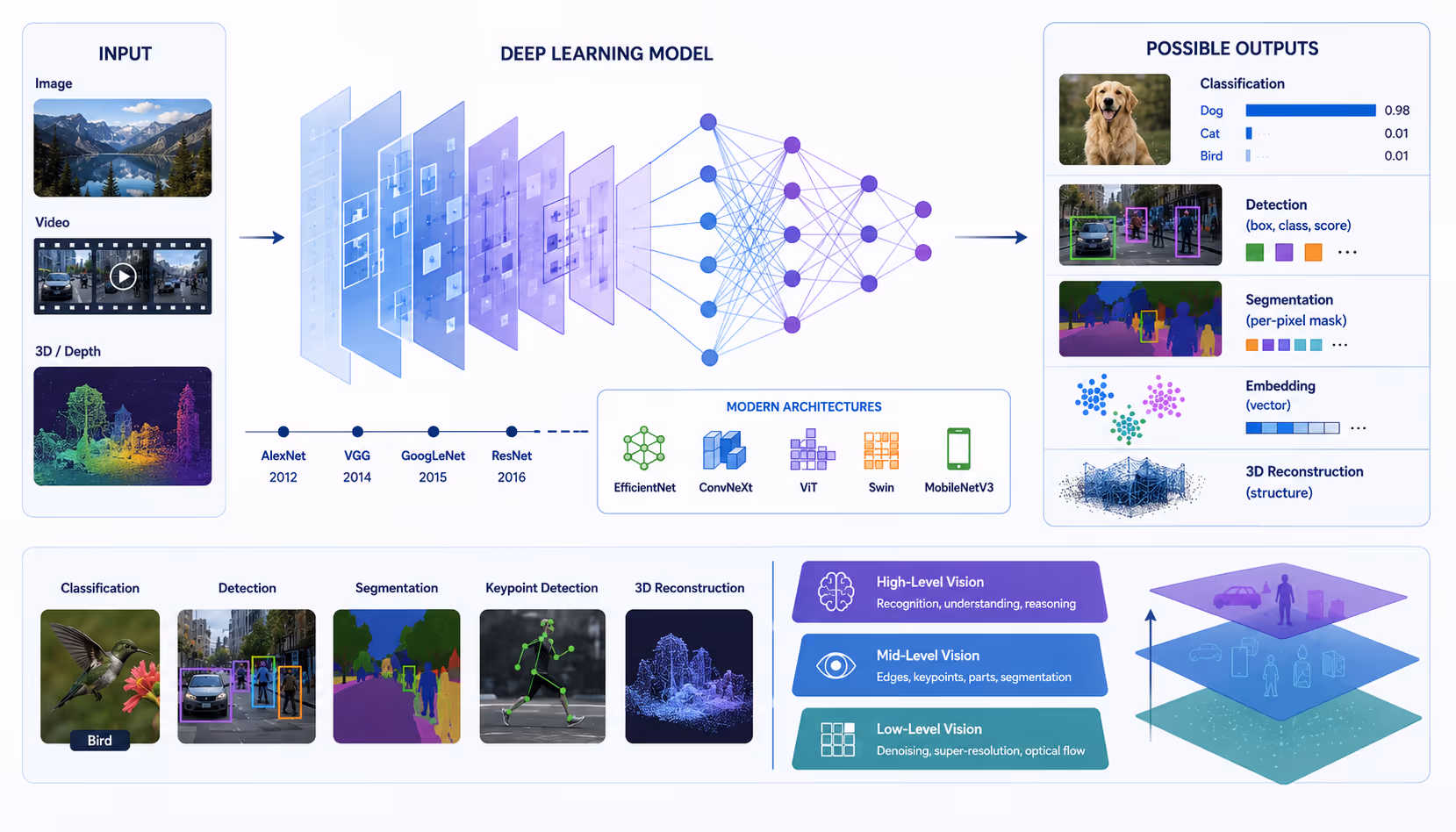
Computer vision is the subfield of artificial intelligence that builds algorithmic systems for acquiring, processing, and reasoning about images, video, and other 2D/3D visual signals. 

Formally, given an image x ∈ ℝ^(H×W×C) (height, width, channels), a CV model implements a function fθ : x → y, where y may be a class label (classification), a set of bounding boxes {(bᵢ, cᵢ, sᵢ)} with class cᵢ and confidence sᵢ (detection), a per-pixel mask (segmentation), an embedding vector (representation learning), or a 3D structure (reconstruction).

Modern CV is dominated by deep learning. The conventional milestone was AlexNet (Krizhevsky et al., 2012), which reduced the ImageNet (Deng et al., 2009; Russakovsky et al., 2015) top-5 error from 26% to 15% using GPU-trained CNNs. Subsequent breakthroughs include VGG (Simonyan & Zisserman, 2015), Inception/GoogLeNet (Szegedy et al., 2015), and ResNet’s residual learning (He et al., 2016), which enabled training of networks with 100+ layers and remains a default classification backbone in 2026, though, importantly, not the only one. 

Production teams today increasingly deploy EfficientNet (Tan & Le, 2019), ConvNeXt (Liu et al., 2022), Vision Transformers (Dosovitskiy et al., 2021), Swin Transformers (Liu et al., 2021), MobileNetV3 (Howard et al., 2019), and MobileViT (Mehta & Rastegari, 2022). VGG, while pedagogically important, is essentially retired from new production work owing to its parameter inefficiency (≈138M parameters at <72% top-1) compared to ConvNeXt-T (≈28M parameters at 82.1%) or ViT-B/16 (≈86M at 84.0% with proper pretraining).

A useful working distinction is low-level vision (denoising, super-resolution, optical flow), mid-level vision (edge/keypoint detection, segmentation), and high-level vision (recognition, scene understanding, VQA). Modern systems compress these layers via end-to-end learning, but the conceptual decomposition remains useful for debugging.

How Computer Vision Works: End-to-End Workflow

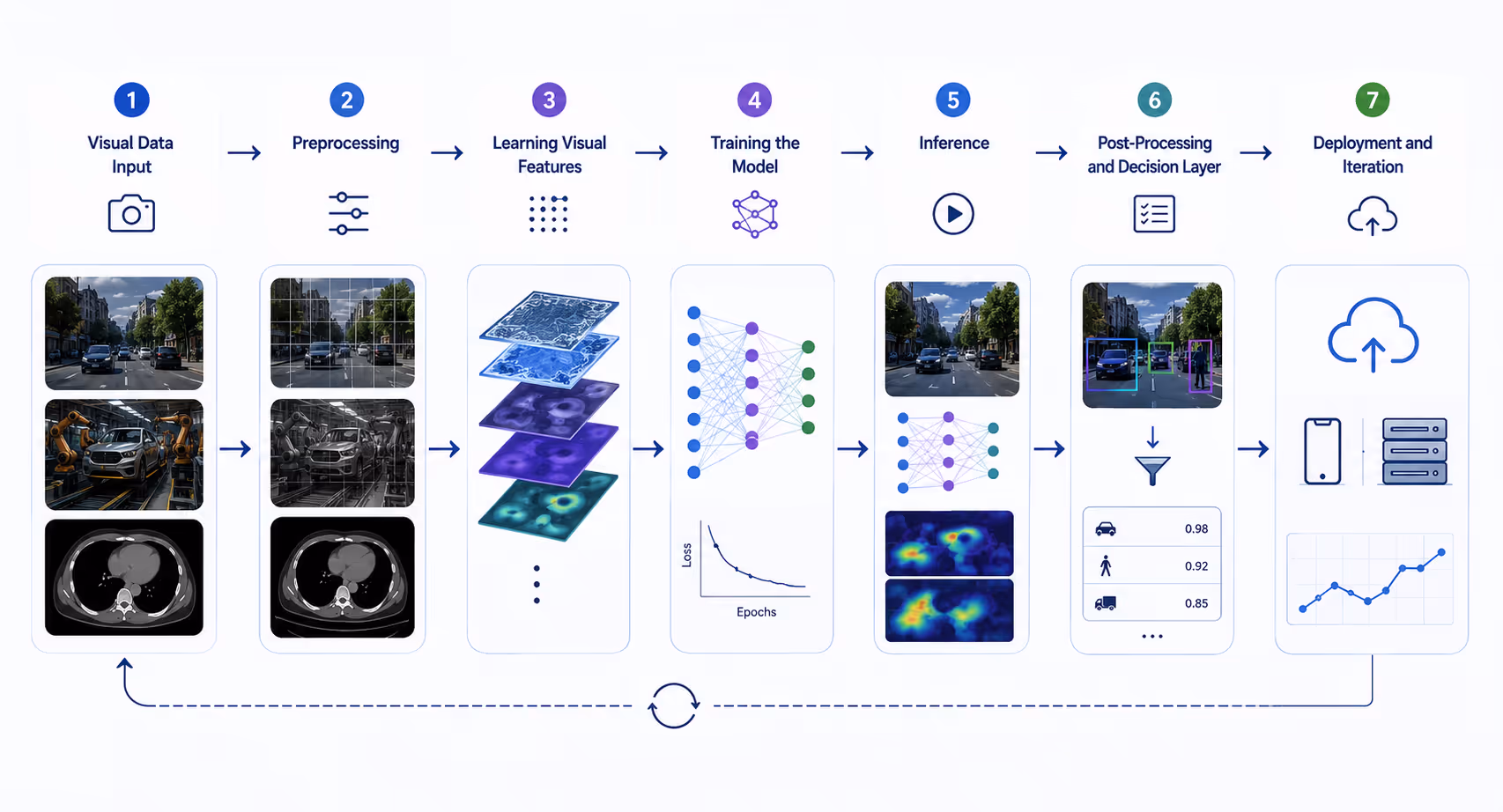
A production computer vision system has seven engineering stages. Treating each as a first-class concern, rather than collapsing them into “train a model,” is what separates research code from systems that survive contact with real users.

1. Visual Data Input

The pipeline begins with image or video acquisition. Source modalities differ enormously in their statistics: 8-bit RGB sensors (sRGB, BT.709), 12–16-bit raw Bayer captures, monochromatic medical DICOM volumes, multi-spectral and hyperspectral satellite imagery, depth maps from structured light or stereo, LiDAR point clouds, and event-camera streams. Each modality has its own noise model (shot, read, fixed-pattern), color space, and dynamic range, and these must be considered before any model design.

For benchmark research, established corpora include ImageNet-21k/1k (Deng et al., 2009; Russakovsky et al., 2015), COCO for detection and segmentation (Lin et al., 2014), Cityscapes for urban semantic segmentation (Cordts et al., 2016), KITTI (Geiger et al., 2012) and Argoverse (Chang et al., 2019) for autonomous driving, MVTec AD for industrial anomaly detection (Bergmann et al., 2019), and ChestX-ray14 (Wang et al., 2017) and the Medical Segmentation Decathlon (Antonelli et al., 2022) for medical imaging. Production data, however, is rarely so clean, class imbalance, distribution shift, and label noise are the dominant pathologies.

2. Preprocessing

Preprocessing normalizes the input distribution and exposes inductive biases through augmentation. Canonical operations include:

• Geometric normalization: resize/crop to network-native resolution (224×224 for most ImageNet-pretrained CNNs and ViTs; 640×640 for YOLO; 800×1333 for Faster R-CNN-style detectors).
• Photometric normalization: subtract per-channel mean and divide by std (ImageNet stats: μ=[0.485, 0.456, 0.406], σ=[0.229, 0.224, 0.225]).
• Augmentation: random crops/flips, color jitter, and modern composite policies — AutoAugment (Cubuk et al., 2019), RandAugment (Cubuk et al., 2020), Mixup (Zhang et al., 2018), CutMix (Yun et al., 2019), and stochastic depth (Huang et al., 2016).

Augmentation acts as data-side regularization. It is conceptually distinct from architectural regularization such as dropout (Srivastava et al., 2014), batch normalization (Ioffe & Szegedy, 2015), L2 weight decay, label smoothing (Szegedy et al., 2016), and early stopping, and effective training recipes typically combine several of these. The original Azumo phrasing of “dropout or regularization” conflates a specific technique with the general category. In practice, dropout is one regularization mechanism among many and is often omitted from ResNet-style networks, where BatchNorm and weight decay suffice.

3. Learning Visual Features

Feature learning is where the architectural choice lives. Three families dominate.

1. Convolutional Neural Networks (CNNs). A CNN applies learnable kernels with local receptive fields and weight sharing, building hierarchical features whose receptive fields progressively expand through depth. Key reference architectures: ResNet (He et al., 2016), DenseNet (Huang et al., 2017), EfficientNet (Tan & Le, 2019), and ConvNeXt (Liu et al., 2022). ConvNeXt-XL achieves 87.8% top-1 on ImageNet-1k with ImageNet-22k pretraining, demonstrating that pure-conv designs remain competitive with transformers when modernized.
2. Vision Transformers (ViTs). Dosovitskiy et al. (2021) split an image into a grid of fixed-size patches (typically 16×16), linearly project each patch to a token embedding, prepend a learnable [CLS] token, add positional embeddings, and run the sequence through a stack of standard Transformer encoder blocks. The contrast with CNNs is not “ViTs see the whole image at once while CNNs see parts,” both ultimately ingest the entire image, but rather that ViT self-attention is global from the very first layer, whereas a CNN’s effective receptive field expands gradually with depth via stacked convolutions and pooling. This has empirical consequences: ViTs are data-hungry (ViT-L/16 underperforms ResNet on ImageNet-1k from scratch but exceeds it after JFT-300M pretraining, Dosovitskiy et al., 2021), more sensitive to optimization recipe, and benefit substantially from hierarchical/window attention (Swin: Liu et al., 2021).
3. Hybrid and convolution-augmented transformers. Swin Transformer (Liu et al., 2021) introduces shifted-window attention that recovers a CNN-like locality and linear-with-image-area complexity, achieving 87.3% top-1 on ImageNet-1k. ConvNeXt (Liu et al., 2022) goes the other direction, modernizing a ResNet with transformer-style design choices (depthwise 7×7 convs, GELU, LayerNorm, fewer activation functions per block), and matches Swin without attention.

Self-supervised foundation models have changed the practical defaults. DINOv2 (Oquab et al., 2024) trains a ViT-g/14 on a curated 142M-image dataset using self-distillation, producing all-purpose features that transfer to classification, segmentation, and depth estimation without finetuning. 

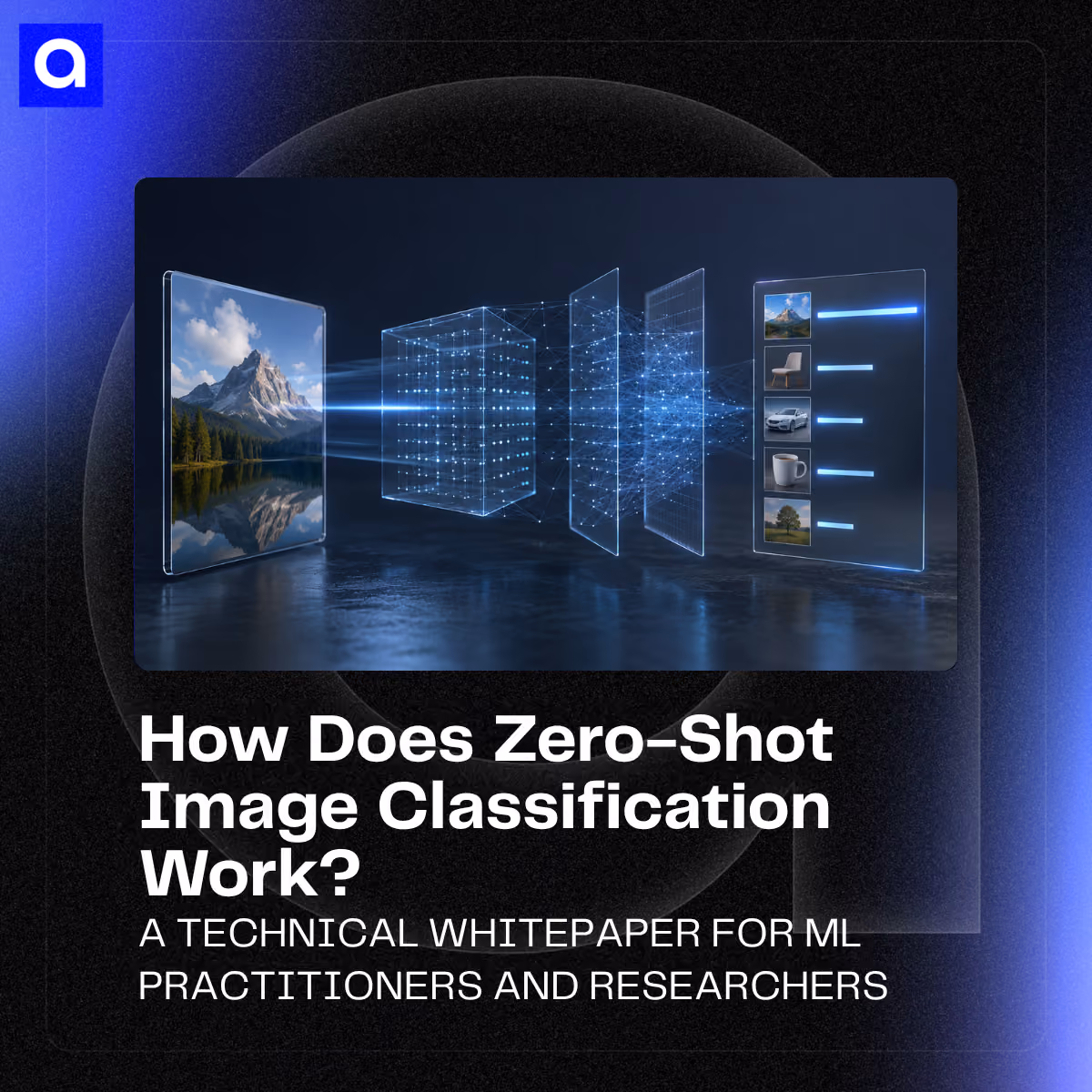
CLIP (Radford et al., 2021) jointly trains image and text encoders contrastively on 400M image–text pairs, enabling zero-shot classification by comparing image embeddings to prompt embeddings (“a photo of a {class}”). Masked Autoencoders (MAE; He et al., 2022), MoCo v3 (Chen et al., 2021), and SimCLR (Chen et al., 2020) round out the self-supervised portfolio. For new projects in 2026, a sensible default is to start from a self-supervised or weakly-supervised checkpoint (DINOv2, CLIP, OpenCLIP, or SAM) rather than from a supervised ImageNet-1k baseline.

4. Training the Model

Training maps a labeled dataset 𝒟 = {(xᵢ, yᵢ)} to parameters θ* = arg minθ 𝔼[𝒛(fθ(x), y)]. The choice of loss is task-dependent:

• Classification: softmax cross-entropy

𝒛_CE = − Σ_{c=1}^{C} y_c · log ŷ_c

often with label smoothing y_c ← (1−ε) y_c + ε/C.

• Detection: a sum of localization (Smooth-L1, IoU, GIoU [Rezatofighi et al., 2019], or DIoU/CIoU [Zheng et al., 2020]) and classification terms; modern DETR-family models (Carion et al., 2020) use Hungarian matching for end-to-end set prediction.
• Semantic segmentation: per-pixel cross-entropy plus Dice loss

𝒛_Dice = 1 − (2·|P ∩ G|) / (|P| + |G|)

which is robust to class imbalance.

• Metric learning: triplet loss (Schroff et al., 2015) or angular-margin losses such as ArcFace (Deng et al., 2019).

Optimization in 2026 is overwhelmingly Adam/AdamW (Kingma & Ba, 2015; Loshchilov & Hutter, 2019) for transformers and SGD with Nesterov momentum for CNN-only stacks, with cosine learning-rate decay (Loshchilov & Hutter, 2017) and linear warmup. The frameworks are PyTorch (Paszke et al., 2019) and TensorFlow (Abadi et al., 2016), supplemented by JAX/Flax for research.

Note*: A critical correction: PyTorch and TensorFlow are training frameworks; they are not experiment-tracking tools. For experiment tracking, lineage, and reproducibility, the standard tooling is MLflow (Zaharia et al., 2018), Weights & Biases, Neptune, or Comet — these capture hyperparameters, metric curves, dataset versions, and model artifacts. Confusing the two leads to ML platforms that train models well but cannot answer “which run produced this checkpoint?” three months later.

Real-world training is dominated by data quality issues, not algorithmic ones. Label noise is pervasive, Northcutt et al. (2021) found average label-error rates of 3.4% across ten widely used benchmarks, including ImageNet, and naïve training on noisy labels leads to memorization and overconfidence. Practical mitigations include confident learning, co-teaching, label cleansing pipelines, and consensus relabeling. Distribution shift between training and deployment data (covariate shift, label shift, concept drift) is a second-order pathology and is often diagnosed only post-deployment through monitoring.

5. Inference

Inference is the forward pass at deployment time. Engineering decisions here have first-order impact on cost and user experience. Key levers:

• Numerical precision: FP32 → FP16/BF16 is typically lossless for modern CNNs and transformers; INT8 post-training quantization (PTQ) with proper calibration usually preserves accuracy within 0.5–1% (Jacob et al., 2018), and INT4 is feasible for some models with quantization-aware training (QAT).
• Compilers: ONNX Runtime, NVIDIA TensorRT, Intel OpenVINO, and Apple Core ML perform graph fusion, kernel selection, and precision lowering.
• Pruning and distillation: unstructured magnitude pruning (Han et al., 2015), structured channel pruning, and knowledge distillation (Hinton et al., 2015) reduce parameters and FLOPs.
• Batching: dynamic batching at the server level amortizes kernel launch overhead but increases tail latency.

For example, a ResNet-50 running TensorRT-INT8 on an NVIDIA T4 achieves >2,000 images/sec at batch=8, versus ~700 images/sec for the PyTorch-FP32 baseline.

6. Post-Processing and Decision Layer

Post-processing converts model logits into actionable outputs:

• Detection: Non-Maximum Suppression (NMS), or its differentiable variants, to remove duplicate boxes; DETR-family models eliminate this step entirely (Carion et al., 2020; Zhao et al., 2024).
• Segmentation: morphological cleanup, connected-component analysis, and CRF refinement (Chen et al., 2018, DeepLabv3+).
• Tracking: SORT, DeepSORT, ByteTrack to associate detections across frames.
• Calibration: temperature scaling (Guo et al., 2017) so that confidence scores reflect empirical accuracy, essential for any system that thresholds or escalates.
• Business logic: thresholding, ROI gating, and human-in-the-loop review for low-confidence predictions.

7. Deployment and Iteration

Deployment splits roughly into cloud, on-premises, and edge. Key trade-offs:

‍

Standard formats, ONNX, TensorRT engines, OpenVINO IR, Core ML, decouple training framework from runtime. Model monitoring (data drift, prediction drift, performance drift) is increasingly handled by tools such as Evidently, Arize, and Fiddler. A/B testing and shadow deployments are how teams roll out new models without regression risk; canary deployments and feature flags are now standard practice.

The platform-language matrix is also worth disambiguating, since the original Azumo article conflated several roles. Python remains the dominant language for training and research. C++ and Rust are common for high-performance inference servers. Java and Kotlin are the canonical languages for Android application code that wraps a TFLite/PyTorch-Mobile/ONNX model. Swift/Objective-C play the analogous role on iOS. MATLAB, by contrast, is used in academic research, signal processing, and certain control-systems pipelines — it is not, in the usual sense, a mobile-development language. Mixing these on a roadmap leads to misaligned hiring and architecture.

Core Computer Vision Techniques 

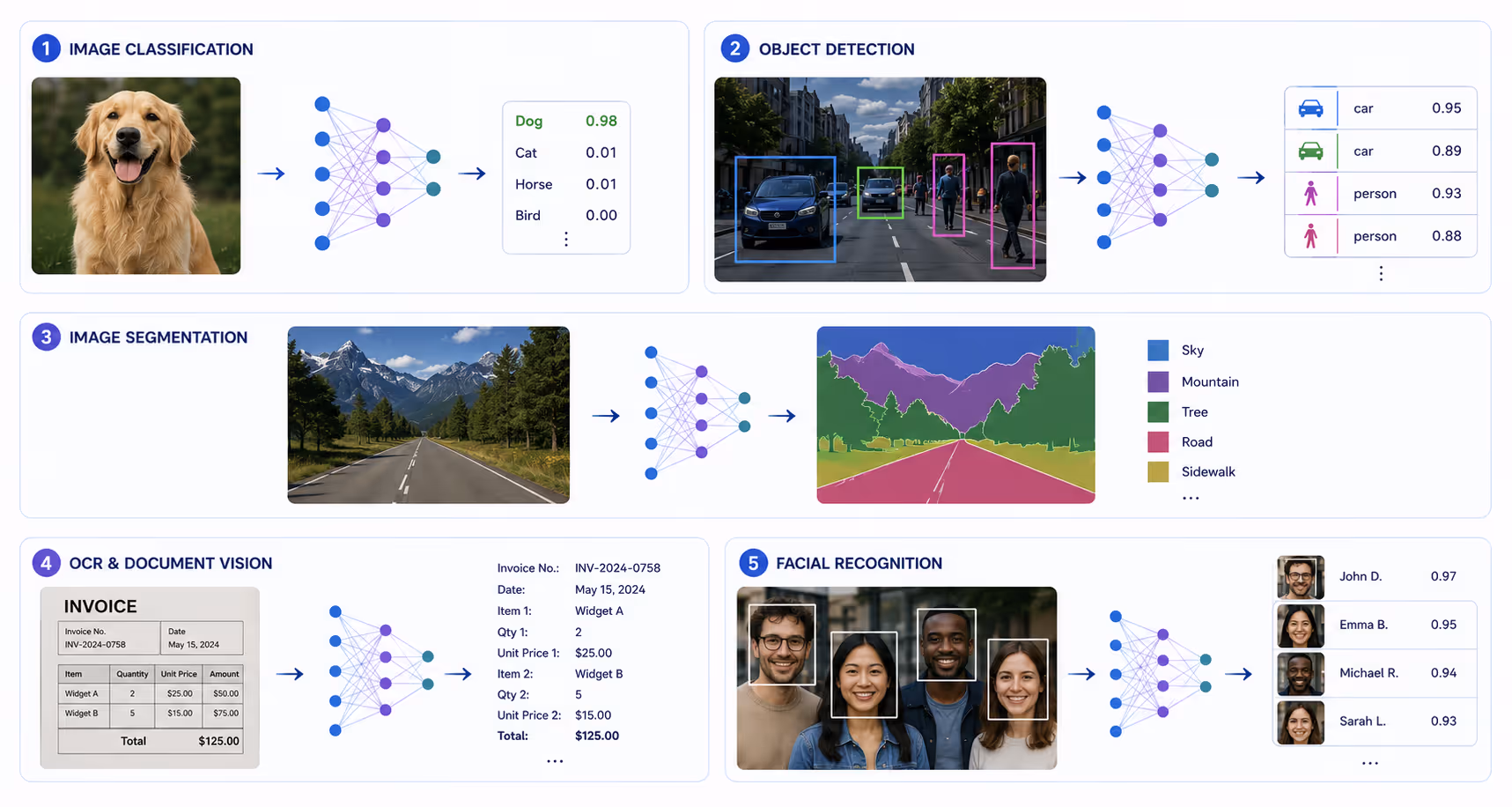
1. Image Classification

Image classification assigns one (or k-of-C) labels to an image. State-of-the-art ImageNet-1k top-1 numbers in 2026 cluster around 88–92% for single-model evaluation, with top results from EVA-02 (Fang et al., 2024), DINOv2-distilled ViTs (Oquab et al., 2024), and BEiT v3 (Wang et al., 2023). Practical defaults:

‍

The cross-entropy loss above remains the canonical training objective; transfer learning from ImageNet-1k or self-supervised checkpoints is universal in industry.

2. Object Detection

Object detection localizes objects via bounding boxes and classifies each box. The reference benchmark is COCO (Lin et al., 2014) with mAP@[0.5:0.95]. The 2015–2018 narrative — “two-stage Faster R-CNN is accurate but slow; one-stage YOLO/SSD is fast but less accurate” — is outdated in 2026. Modern one-stage and DETR-style detectors meet or beat the original Faster R-CNN at substantially higher FPS:

‍

Note*: YOLOv10-S: 1.8× faster than RT-DETR-R18 at similar AP per Wang et al. (2024b). FPS numbers are approximate and from the original papers’ T4 FP16 benchmarks; treat as illustrative rather than directly comparable across compilation toolchains.

The takeaway is twofold. First, modern YOLO variants and RT-DETR dominate the latency–accuracy Pareto frontier, frequently surpassing Faster R-CNN’s accuracy at 3–5× higher throughput on the same hardware. Second, the choice between YOLO and DETR-family detectors is no longer about accuracy ceilings but about engineering preferences: DETR removes NMS (a non-trivial deployment win for end-to-end pipelines and ONNX export) at the cost of higher training iteration counts and harder small-object regimes; YOLOs remain marginally simpler to fine-tune. Faster R-CNN persists primarily in legacy systems and certain academic baselines.

A frequent source of confusion in transfer-learning discussions is treating “ResNet” and “YOLO” as interchangeable starting points. They are not. ResNet is a backbone (feature extractor) used inside detection, segmentation, and classification systems; YOLO is a complete detection architecture (backbone + neck + head + loss). When practitioners “fine-tune YOLO,” they fine-tune the entire detector; when they “fine-tune ResNet,” they typically fine-tune a classifier head on top of frozen or partially-unfrozen ResNet features — or use ResNet as the backbone within a larger system (e.g., Faster R-CNN with ResNet-50-FPN).

3. Image Segmentation

Image segmentation produces a label per pixel (semantic), per pixel-and-instance (instance), or per pixel-instance-and-stuff (panoptic).

• Semantic segmentation: U-Net (Ronneberger et al., 2015), the DeepLab series (Chen et al., 2018), SegFormer (Xie et al., 2021), Mask2Former (Cheng et al., 2022). Standard benchmarks: Cityscapes (mIoU), ADE20K, Pascal VOC.
• Instance segmentation: Mask R-CNN (He et al., 2017) extends Faster R-CNN with a mask branch and remains a strong baseline at ~37.1% mask AP on COCO. YOLACT (Bolya et al., 2019) and CondInst (Tian et al., 2020) trade some accuracy for real-time inference. Canonical use cases include separating people in a crowded scene, individual cars in a parking lot, or each fruit on a conveyor belt, well-defined, mostly non-overlapping instances.
• Panoptic segmentation: unifies “things” (instances) and “stuff” (sky, road) into one map; Mask2Former (Cheng et al., 2022) handles all three regimes within one architecture.
• Foundation segmentation: SAM (Kirillov et al., 2023) is a promptable segmentation model trained on 1B+ masks, enabling zero-shot segmentation given a point, box, or mask prompt. SAM 2 (Ravi et al., 2024) extends this to video with a streaming-memory transformer, enabling real-time promptable video segmentation while remaining 6× faster than SAM on still images.
• Medical imaging: nnU-Net (Isensee et al., 2021) is a self-configuring U-Net pipeline that auto-tunes preprocessing, architecture, and training for each new task; it has won or placed in 23+ international medical segmentation challenges and remains the strongest out-of-the-box choice for new modalities.

The Dice loss formulation introduced earlier is dominant for medical segmentation; combinations of Dice + cross-entropy + boundary-aware terms are typical.

4. OCR and Document Vision

Document vision blends classical OCR with modern multimodal modeling:

• Detection–recognition pipelines: EAST (Zhou et al., 2017) or DBNet (Liao et al., 2020) for text detection, followed by CRNN (Shi et al., 2017) or attention-based recognizers.
• Transformer OCR: TrOCR (Li et al., 2023) treats OCR as image-to-text generation with a ViT encoder and a text decoder, achieving SOTA on SROIE and IAM.
• Document understanding: LayoutLM v1/v2/v3 (Xu et al., 2020; Xu et al., 2022) jointly models text, layout, and image features for tasks such as form understanding, receipt extraction, and table parsing. Donut (Kim et al., 2022) eschews OCR entirely and reads documents end-to-end with a transformer, useful when OCR errors propagate downstream.

Production document-AI systems typically combine a document-region detector, a recognizer, a layout model, and a structured-extraction stage with explicit business-rule validation.

5. Facial Recognition

Face recognition splits into detection (RetinaFace; Deng et al., 2020), alignment, embedding, and matching. The dominant embedding paradigm is metric learning with angular margins:

• FaceNet (Schroff et al., 2015) introduced triplet loss for 128-D face embeddings.
• ArcFace (Deng et al., 2019) added an additive angular margin:

𝒛 = − log [ e^{s·cos(θ_yi + m)} / ( e^{s·cos(θ_yi + m)} + Σ_{j≠yi} e^{s·cosθ_j} ) ]

achieving 99.83% on LFW and significantly better discrimination on MegaFace.

Facial recognition is also the most ethically loaded CV application. Deployments must address demographic bias (Buolamwini & Gebru, 2018), consent, retention policy, and jurisdictional legality (EU AI Act high-risk classification, GDPR, US state laws). These are not afterthoughts.

Where Is Computer Vision Used?

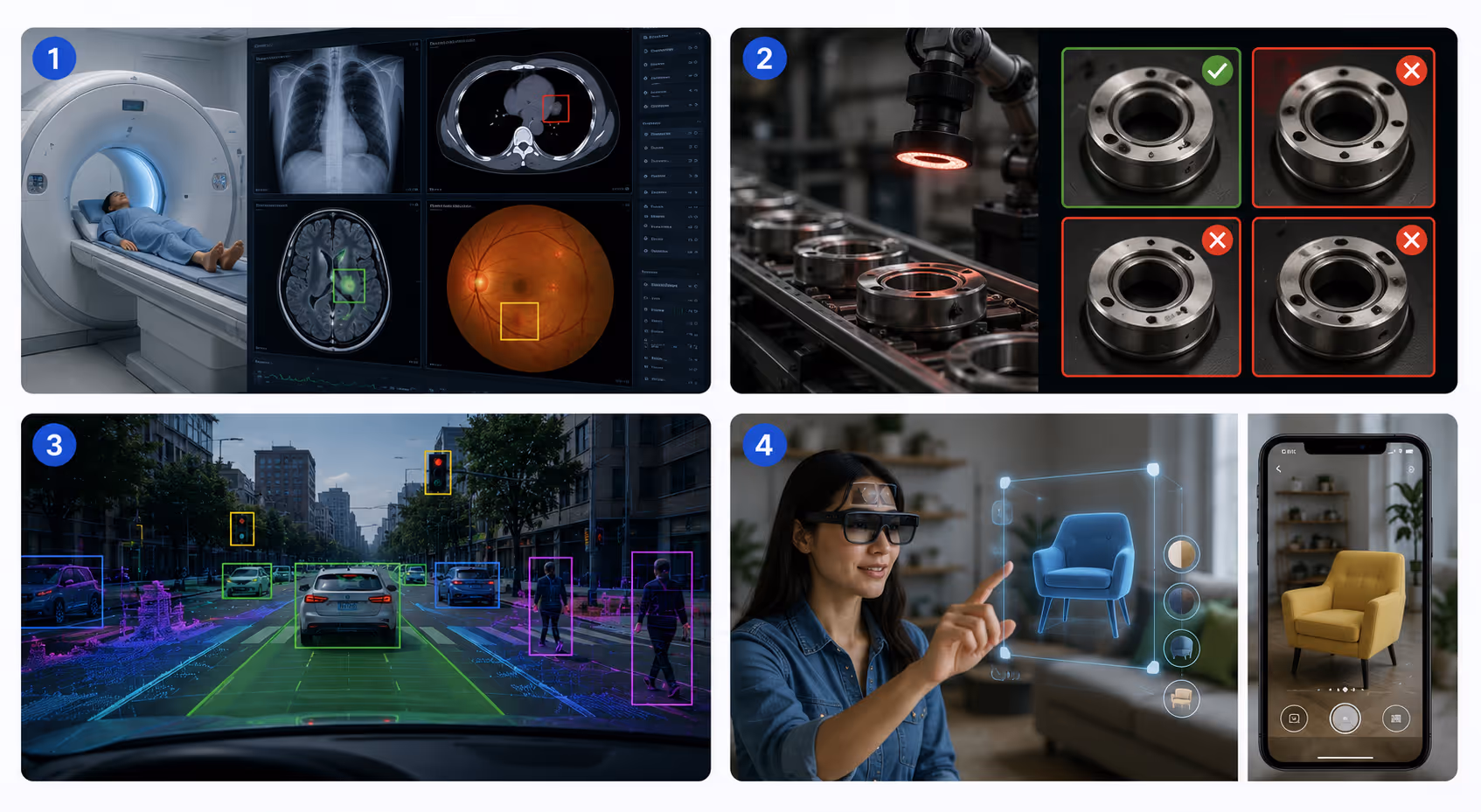
1. Medical Imaging and Healthcare

Medical imaging is the highest-stakes, highest-rigor application domain. Landmark studies include:

• Diabetic retinopathy: Gulshan et al. (2016) demonstrated, in JAMA, a deep-learning algorithm for grading retinal fundus photographs that achieved 0.991 AUC for referable DR, comparable to board-certified ophthalmologists.
• Pneumonia detection: CheXNet (Rajpurkar et al., 2017), a 121-layer DenseNet trained on ChestX-ray14, exceeded average radiologist F1 on pneumonia detection from chest radiographs.
• Skin cancer: Esteva et al. (2017) showed dermatologist-level keratinocyte and melanoma classification from clinical images.
• Pathology: Campanella et al. (2019) demonstrated clinical-grade whole-slide cancer detection at scale.
• Volumetric segmentation: nnU-Net (Isensee et al., 2021) is the de facto baseline for organ and tumor segmentation across CT and MRI modalities.

Medical CV systems require regulatory approval (FDA 510(k) / De Novo / PMA, CE mark under EU MDR), validated clinical workflows, prospective external validation (not just retrospective held-out test sets), and rigorous calibration. Distribution shift across hospitals, scanners, and protocols is the single largest source of real-world failure.

2. Defect Detection and Quality Control

Visual inspection is a core Industry-4.0 application and a frequent first computer-vision project. The standard public benchmark is MVTec AD (Bergmann et al., 2019), comprising 5,354 high-resolution images across 15 object/texture classes with pixel-level anomaly annotations; modern methods such as PatchCore (Roth et al., 2022) and EfficientAD achieve >99% image-level AUROC on most categories.

When discussing impact, it is important to use parallel framings rather than mixed metrics. For example: “manual inspection commonly achieves 70–80% defect-detection recall; production CV systems with proper calibration commonly achieve 98–99% recall on the same defect class at controlled false-positive rates” — as opposed to mixing miss-rate (“misses 20–30%”) with detection-rate (“98–99% detection”), which superficially compare apples to oranges.

Engineering specifics: lighting and fixturing dominate accuracy (a properly lit conveyor often does more than a deeper model); few-shot anomaly detection (Roth et al., 2022; Bergmann et al., 2019) lets teams deploy with as few as a handful of normal examples; and edge deployment on Jetson-class hardware at 30+ FPS is typical for line-rate inspection.

3. Self-Driving and Autonomy

Autonomous-vehicle (AV) perception is a multi-sensor problem. The frequent error of describing “CV combined with LiDAR and RADAR to detect lanes, identify pedestrians, and read traffic signs” obscures what each sensor actually does. A correct decomposition:

• Cameras + CV — the only modality that delivers dense semantic content: traffic-sign and traffic-light classification and text reading, lane-marking detection, free-space segmentation, and fine-grained object classification. Reading a “STOP” sign or a 35 mph speed-limit numeral requires high-resolution imagery and OCR/classification — LiDAR and radar cannot do this.
• LiDAR — accurate 3D distance and geometry through point clouds. Models include PointNet/PointNet++ (Qi et al., 2017a, 2017b), VoxelNet (Zhou & Tuzel, 2018), PointPillars (Lang et al., 2019), and CenterPoint (Yin et al., 2021).
• Radar — robust velocity (Doppler) and range, especially in adverse weather (rain, fog) where cameras and LiDAR degrade.
• Sensor fusion — early, mid, or late fusion combines the modalities; recent BEV-based methods such as BEVFormer (Li et al., 2022) and TransFusion (Bai et al., 2022) operate in a unified bird’s-eye-view space.

The end-to-end perception → prediction → planning → control pipeline is what must meet real-time constraints. Per-frame perception on a modern AV stack typically runs in 20–60 ms on the AV-grade compute (e.g., NVIDIA Drive Orin, custom Tesla FSD Computer); the full perception → decision → actuation cycle is more typically in the 100–300 ms range, and streaming-perception research (Li, Wang & Ramanan, ECCV 2020) has shown that end-to-end streaming AP — which accounts for the world having moved while the model was thinking — drops substantially when latency is ignored. Stating that “AVs process each frame in 50–200 ms” is therefore both ambiguous (perception alone vs. full loop) and on the slow side of acceptable for safety-critical perception. Modern systems aim for ≤50 ms perception with explicit latency-aware metrics (Argoverse-HD streaming AP).

4. AR and Interactive Experiences

Augmented reality stitches CV with real-time graphics:

• SLAM (simultaneous localization and mapping): ORB-SLAM3 (Campos et al., 2021) provides robust visual-inertial SLAM and is a common baseline; commercial AR (Apple ARKit, Google ARCore, Meta) layers proprietary improvements.
• Pose and hand tracking: MediaPipe and similar pipelines run real-time landmark estimation on mobile.
• Novel view synthesis: NeRF (Mildenhall et al., 2020) introduced volumetric implicit representations of 3D scenes; 3D Gaussian Splatting (Kerbl et al., SIGGRAPH 2023) replaced costly volume marching with rasterized anisotropic Gaussians, enabling real-time (≥30 FPS, often >100 FPS) 1080p novel-view rendering. Both are now standard tools in AR/VR content pipelines and digital-twin reconstruction.
• Foundation video models: SAM 2 (Ravi et al., 2024) provides promptable video segmentation suitable for AR object isolation.

How Azumo Helps Teams Implement Computer Vision

Azumo provides computer vision development, including the creation of production-grade computer vision systems across object detection, classification, video analytics, OCR, and visual inspection. Their delivery model pairs senior ML engineers with clients in manufacturing, healthcare, retail, and logistics. Typical engagements cover the full lifecycle described in §3: data assessment and annotation strategy, model architecture selection (ResNet/EfficientNet/ViT for classification; YOLO and RT-DETR for detection; nnU-Net / SAM 2 for segmentation), MLOps tooling (MLflow, Weights & Biases for tracking; ONNX, TensorRT, OpenVINO for deployment), and post-deployment monitoring.

References

• Abadi, M., et al. (2016). TensorFlow: A system for large-scale machine learning. OSDI ’16.
• Antonelli, M., et al. (2022). The Medical Segmentation Decathlon. Nature Communications, 13, 4128.
• Bai, X., et al. (2022). TransFusion: Robust LiDAR–Camera Fusion for 3D Object Detection with Transformers. CVPR 2022.
• Bergmann, P., Fauser, M., Sattlegger, D., & Steger, C. (2019). MVTec AD — A Comprehensive Real-World Dataset for Unsupervised Anomaly Detection. CVPR 2019, 9592–9600.
• Bolya, D., et al. (2019). YOLACT: Real-time Instance Segmentation. ICCV 2019.
• Buolamwini, J., & Gebru, T. (2018). Gender Shades: Intersectional Accuracy Disparities in Commercial Gender Classification. FAT* 2018.
• Campanella, G., et al. (2019). Clinical-grade computational pathology using weakly supervised deep learning on whole slide images. Nature Medicine, 25, 1301–1309.
• Campos, C., et al. (2021). ORB-SLAM3: An Accurate Open-Source Library for Visual, Visual–Inertial, and Multimap SLAM. IEEE T-RO, 37(6).
• Carion, N., et al. (2020). End-to-End Object Detection with Transformers. ECCV 2020. arXiv:2005.12872.
• Chang, M.-F., et al. (2019). Argoverse: 3D Tracking and Forecasting with Rich Maps. CVPR 2019.
• Chen, L.-C., et al. (2018). Encoder–Decoder with Atrous Separable Convolution for Semantic Image Segmentation (DeepLabv3+). ECCV 2018.
• Chen, T., Kornblith, S., Norouzi, M., & Hinton, G. (2020). A Simple Framework for Contrastive Learning of Visual Representations (SimCLR). ICML 2020.
• Chen, X., Xie, S., & He, K. (2021). An Empirical Study of Training Self-Supervised Vision Transformers (MoCo v3). ICCV 2021.
• Cheng, B., et al. (2022). Masked-attention Mask Transformer for Universal Image Segmentation (Mask2Former). CVPR 2022.
• Cordts, M., et al. (2016). The Cityscapes Dataset for Semantic Urban Scene Understanding. CVPR 2016.
• Cubuk, E. D., et al. (2019). AutoAugment: Learning Augmentation Strategies from Data. CVPR 2019.
• Cubuk, E. D., et al. (2020). RandAugment: Practical Automated Data Augmentation with a Reduced Search Space. NeurIPS 2020 Workshops.
• Deng, J., et al. (2009). ImageNet: A Large-Scale Hierarchical Image Database. CVPR 2009.
• Deng, J., et al. (2019). ArcFace: Additive Angular Margin Loss for Deep Face Recognition. CVPR 2019. arXiv:1801.07698.
• Deng, J., et al. (2020). RetinaFace: Single-shot Multi-level Face Localisation in the Wild. CVPR 2020.
• Dosovitskiy, A., et al. (2021). An Image is Worth 16×16 Words: Transformers for Image Recognition at Scale. ICLR 2021. arXiv:2010.11929.
• Esteva, A., et al. (2017). Dermatologist-level classification of skin cancer with deep neural networks. Nature, 542, 115–118.
• Fang, Y., et al. (2024). EVA-02: A Visual Representation for Neon Genesis. Image and Vision Computing.
• Geiger, A., Lenz, P., & Urtasun, R. (2012). Are we ready for autonomous driving? The KITTI vision benchmark suite. CVPR 2012.
• Grand View Research. (2025). Computer Vision Market Size, Share & Trends Report, 2025–2030. Industry report.
• Gulshan, V., et al. (2016). Development and Validation of a Deep Learning Algorithm for Detection of Diabetic Retinopathy in Retinal Fundus Photographs. JAMA, 316(22), 2402–2410.
• Guo, C., et al. (2017). On Calibration of Modern Neural Networks. ICML 2017.
• Han, S., Mao, H., & Dally, W. (2015). Deep Compression: Compressing Deep Neural Networks with Pruning, Trained Quantization and Huffman Coding. ICLR 2016.
• He, K., Zhang, X., Ren, S., & Sun, J. (2016). Deep Residual Learning for Image Recognition. CVPR 2016. arXiv:1512.03385.
• He, K., et al. (2017). Mask R-CNN. ICCV 2017. arXiv:1703.06870.
• He, K., et al. (2022). Masked Autoencoders Are Scalable Vision Learners. CVPR 2022.
• Hinton, G., Vinyals, O., & Dean, J. (2015). Distilling the Knowledge in a Neural Network. arXiv:1503.02531.
• Howard, A., et al. (2019). Searching for MobileNetV3. ICCV 2019.
• Huang, G., et al. (2016). Deep Networks with Stochastic Depth. ECCV 2016.
• Huang, G., et al. (2017). Densely Connected Convolutional Networks. CVPR 2017.
• Ioffe, S., & Szegedy, C. (2015). Batch Normalization: Accelerating Deep Network Training by Reducing Internal Covariate Shift. ICML 2015.
• Isensee, F., Jaeger, P. F., Kohl, S. A. A., Petersen, J., & Maier-Hein, K. H. (2021). nnU-Net: a self-configuring method for deep learning-based biomedical image segmentation. Nature Methods, 18, 203–211.
• Jacob, B., et al. (2018). Quantization and Training of Neural Networks for Efficient Integer-Arithmetic-Only Inference. CVPR 2018.
• Jocher, G., et al. (2023). YOLOv8 by Ultralytics. https://github.com/ultralytics/ultralytics.
• Kerbl, B., Kopanas, G., Leimkühler, T., & Drettakis, G. (2023). 3D Gaussian Splatting for Real-Time Radiance Field Rendering. ACM Trans. Graph. (SIGGRAPH 2023), 42(4).
• Kim, G., et al. (2022). OCR-free Document Understanding Transformer (Donut). ECCV 2022.
• Kingma, D. P., & Ba, J. (2015). Adam: A Method for Stochastic Optimization. ICLR 2015.
• Kirillov, A., et al. (2023). Segment Anything. ICCV 2023. arXiv:2304.02643.
• Krizhevsky, A., Sutskever, I., & Hinton, G. (2012). ImageNet Classification with Deep Convolutional Neural Networks. NeurIPS 2012.
• Lang, A. H., et al. (2019). PointPillars: Fast Encoders for Object Detection from Point Clouds. CVPR 2019.
• Li, M., Wang, Y.-X., & Ramanan, D. (2020). Towards Streaming Perception. ECCV 2020.
• Li, M., et al. (2023). TrOCR: Transformer-based Optical Character Recognition with Pre-trained Models. AAAI 2023. arXiv:2109.10282.
• Li, Z., et al. (2022). BEVFormer: Learning Bird’s-Eye-View Representation from Multi-Camera Images via Spatiotemporal Transformers. ECCV 2022.
• Liao, M., et al. (2020). Real-time Scene Text Detection with Differentiable Binarization (DBNet). AAAI 2020.
• Lin, T.-Y., et al. (2014). Microsoft COCO: Common Objects in Context. ECCV 2014.
• Liu, W., et al. (2016). SSD: Single Shot MultiBox Detector. ECCV 2016.
• Liu, Z., et al. (2021). Swin Transformer: Hierarchical Vision Transformer using Shifted Windows. ICCV 2021. arXiv:2103.14030.
• Liu, Z., et al. (2022). A ConvNet for the 2020s (ConvNeXt). CVPR 2022. arXiv:2201.03545.
• Loshchilov, I., & Hutter, F. (2017). SGDR: Stochastic Gradient Descent with Warm Restarts. ICLR 2017.
• Loshchilov, I., & Hutter, F. (2019). Decoupled Weight Decay Regularization (AdamW). ICLR 2019.
• Mehta, S., & Rastegari, M. (2022). MobileViT: Light-weight, General-purpose, and Mobile-friendly Vision Transformer. ICLR 2022.
• Mildenhall, B., et al. (2020). NeRF: Representing Scenes as Neural Radiance Fields for View Synthesis. ECCV 2020.
• Northcutt, C. G., Athalye, A., & Mueller, J. (2021). Pervasive Label Errors in Test Sets Destabilize Machine Learning Benchmarks. NeurIPS Datasets & Benchmarks Track.
• Oquab, M., et al. (2024). DINOv2: Learning Robust Visual Features without Supervision. Transactions on Machine Learning Research. arXiv:2304.07193.
• Paszke, A., et al. (2019). PyTorch: An Imperative Style, High-Performance Deep Learning Library. NeurIPS 2019.
• Qi, C. R., et al. (2017a). PointNet: Deep Learning on Point Sets for 3D Classification and Segmentation. CVPR 2017.
• Qi, C. R., et al. (2017b). PointNet++: Deep Hierarchical Feature Learning on Point Sets in a Metric Space. NeurIPS 2017.
• Radford, A., et al. (2021). Learning Transferable Visual Models From Natural Language Supervision (CLIP). ICML 2021. arXiv:2103.00020.
• Rajpurkar, P., et al. (2017). CheXNet: Radiologist-Level Pneumonia Detection on Chest X-Rays with Deep Learning. arXiv:1711.05225.
• Ravi, N., et al. (2024). SAM 2: Segment Anything in Images and Videos. arXiv:2408.00714.
• Redmon, J., et al. (2016). You Only Look Once: Unified, Real-Time Object Detection. CVPR 2016. arXiv:1506.02640.
• Redmon, J., & Farhadi, A. (2018). YOLOv3: An Incremental Improvement. arXiv:1804.02767.
• Ren, S., He, K., Girshick, R., & Sun, J. (2015). Faster R-CNN: Towards Real-Time Object Detection with Region Proposal Networks. NeurIPS 2015. arXiv:1506.01497.
• Rezatofighi, H., et al. (2019). Generalized Intersection over Union: A Metric and a Loss for Bounding Box Regression. CVPR 2019.
• Ronneberger, O., Fischer, P., & Brox, T. (2015). U-Net: Convolutional Networks for Biomedical Image Segmentation. MICCAI 2015. arXiv:1505.04597.
• Roth, K., et al. (2022). Towards Total Recall in Industrial Anomaly Detection (PatchCore). CVPR 2022.
• Russakovsky, O., et al. (2015). ImageNet Large Scale Visual Recognition Challenge. IJCV, 115(3), 211–252.
• Schroff, F., Kalenichenko, D., & Philbin, J. (2015). FaceNet: A Unified Embedding for Face Recognition and Clustering. CVPR 2015. arXiv:1503.03832.
• Shi, B., Bai, X., & Yao, C. (2017). An End-to-End Trainable Neural Network for Image-Based Sequence Recognition (CRNN). IEEE TPAMI.
• Simonyan, K., & Zisserman, A. (2015). Very Deep Convolutional Networks for Large-Scale Image Recognition (VGG). ICLR 2015. arXiv:1409.1556.
• Srivastava, N., et al. (2014). Dropout: A Simple Way to Prevent Neural Networks from Overfitting. JMLR, 15, 1929–1958.
• Szegedy, C., et al. (2015). Going Deeper with Convolutions (GoogLeNet). CVPR 2015.
• Szegedy, C., et al. (2016). Rethinking the Inception Architecture for Computer Vision. CVPR 2016.
• Tan, M., & Le, Q. V. (2019). EfficientNet: Rethinking Model Scaling for Convolutional Neural Networks. ICML 2019. arXiv:1905.11946.
• Tian, Z., Shen, C., & Chen, H. (2020). Conditional Convolutions for Instance Segmentation (CondInst). ECCV 2020.
• Wang, C.-Y., Yeh, I.-H., & Liao, H.-Y. M. (2024a). YOLOv9: Learning What You Want to Learn Using Programmable Gradient Information. arXiv:2402.13616.
• Wang, A., et al. (2024b). YOLOv10: Real-Time End-to-End Object Detection. NeurIPS 2024. arXiv:2405.14458.
• Wang, W., et al. (2023). Image as a Foreign Language: BEiT Pretraining for All Vision and Vision–Language Tasks (BEiT v3). CVPR 2023.
• Wang, X., et al. (2017). ChestX-ray8: Hospital-scale Chest X-ray Database and Benchmarks on Weakly-Supervised Classification. CVPR 2017.
• Xie, E., et al. (2021). SegFormer: Simple and Efficient Design for Semantic Segmentation with Transformers. NeurIPS 2021.
• Xu, Y., et al. (2020). LayoutLM: Pre-training of Text and Layout for Document Image Understanding. KDD 2020.
• Xu, Y., et al. (2022). LayoutLMv3: Pre-training for Document AI with Unified Text and Image Masking. ACM MM 2022.
• Yin, T., Zhou, X., & Krähenbühl, P. (2021). Center-based 3D Object Detection and Tracking (CenterPoint). CVPR 2021.
• Yun, S., et al. (2019). CutMix: Regularization Strategy to Train Strong Classifiers with Localizable Features. ICCV 2019.
• Zaharia, M., et al. (2018). Accelerating the Machine Learning Lifecycle with MLflow. IEEE Data Eng. Bull..
• Zhang, H., et al. (2018). mixup: Beyond Empirical Risk Minimization. ICLR 2018. arXiv:1710.09412.
• Zhao, Y., Lv, W., Xu, S., Wei, J., Wang, G., Dang, Q., Liu, Y., & Chen, J. (2024). DETRs Beat YOLOs on Real-time Object Detection (RT-DETR). CVPR 2024, 16965–16974. arXiv:2304.08069.
• Zheng, Z., et al. (2020). Distance-IoU Loss: Faster and Better Learning for Bounding Box Regression. AAAI 2020.
• Zhou, X., & Tuzel, O. (2018). VoxelNet: End-to-End Learning for Point Cloud Based 3D Object Detection. CVPR 2018.
• Zhou, X., et al. (2017). EAST: An Efficient and Accurate Scene Text Detector. CVPR 2017.
• Zhu, X., et al. (2021). Deformable DETR: Deformable Transformers for End-to-End Object Detection. ICLR 2021.

Note*: Authored as a technical reference for ML engineers and researchers. Benchmark numbers are drawn from the cited primary papers; FPS figures were measured on NVIDIA T4 with FP16/TensorRT in the original publications and may differ on alternative compilation toolchains. All cited papers were verified at arXiv, the CVF Open Access archive, Nature/JAMA, and venue proceedings prior to publication.